|
Bridging Functional and Structural Brain Connectivity
Vision of the Project
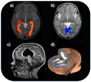 |
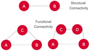
a) Probabilistic tractography reveals a structural pathway between the lateral geniculate nucleus of the thalamus and the visual cortex. b) Functional imaging reveals activation of the visual areas in the same healthy subject. c) Shows a unilateral lesion, and d) The analysis of the structural and functional connectivity reveals that both function and structure is disrupted in the hemisphere with the lesion.
© Hammersmith Hospital, Imperial College London. (Kindly provided by Prof. A. David Edwards).
|
The brain's computation power and stability depends critically on connectivity, which governs the dynamics of signal transfer from one area to another. In fact, disturbances of brain connectivity have been implicated in a number of diseases including schizophrenia attention eficit hyperactivity disorder (ADHD), autism, alzheimer disease (AD), stroke and brain trauma. This has resulted in recent interest in network organisation and dynamics. Magnetic Resonance Imaging (MRI) can be used to derive structural and functional brain networks from diffusion weighted MRI (DWI) and resting-state functional MRI (rs-fMRI). Several tractography techniques have been developed that exploit voxel-based directional information to extract structural networks from DWI. On the other hand, functional networks are defined based on the temporal correlations between spatially remote neurophysiological events. Integrating measures of structural and functional brain connectivity holds the promise of dramatically improving our understanding of brain function and malfunction and could lead to the development of clinically useful biomarkers.
The vision of this project is to map structural abnormalities into functional networks and provide insight on how structure affects function and vice versa. Both the benefits and the challenges of this problem are tremendous. Firstly, rs-fMRI and DWI are indirect measures of function and structure, respectively. Secondly, the complexity of the problem increases exponentially with the number of brain regions. My work suggests the following approaches to regularise the problem:
utilise a prediction modeling of functional connectivity from structural connectivity. This uses out-of-sample error to select the best performing model. This is a measure on how the model will generalise to an independent data set.
extract a sparse representation of structural connectivity to limit model complexity and remove connections that are noisy and irrelevant,
consider the functional connectivity matrices as multivariate objects and hence, constrain the predicted pair-wise functional connections into the space of symmetric positive definite matrices.
utilise a generative model of rs-fMRI data based on Gaussian graphical models to describe conditional dependencies between time-series, and
use randomized lasso to provide a robust fit for correlated predictors (structural connections) and a statistical control over false positives.
Objectives
It is well accepted that functional connectivity and structural brain connectivity are interlinked and they are both affected in neurological diseases. It has been also shown that strong structural connections are typically associated with strong functional connections between regions. Given a set of ROIs and the associated connections between each pair of ROIs we would like to construct a systematic framework to characterise the link between functional and structural connectivity and answer the following questions.
Can we predict changes in functional connectivity from changes in structural connectivity? Then we could potentially estimate the functional dysfunction once we have identified structural abnormalities.
Can we identify reliably the structural connections that affect a specific functional connection and isolate the effect that one connection has on another? Then we can invalidate causal alternatives and help researchers in choosing between competing theories.
Can we answer these questions with a rigorous statistical framework? Then we can generalise our conclusions from a sample set of subjects to the general population.
Basics in Neuroimaging and Brain Connectivity
Brain Organisation
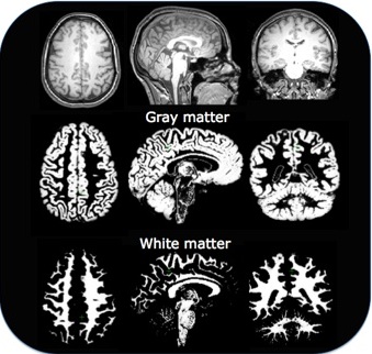
Brain organisation resembles a network that connects areas, which constitute functional units and they are typically specialised to a specific function. These areas consist of neuronal cell bodies, whereas the wiring of the brain is accomplished via neuronal axons. Cytoarchitecture of these areas are fundamentally different, which results in different tissue properties and thus different colours on medical images. Neuronal bodies are usually located in grey matter, which has gray color on T1 MRI images. Neuronal axons are located in white matter, which has brighter color on the same images and hence it can be distinguished. This process is called tissue segmentation and it requires sophisticated computational techniques.
Brain connectivity
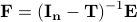
Brain connectivity refers to how functionally specialised units interact with each other. It encompasses both the network's architecture as well as the network dynamics associated with brain function.
In living human brain, network organisation can be described based on diffusion weighted MRI (DWI). Brain function is usually measured with fMRI. Both imaging techniques provide indirect estimations of brain structure and function, respectively. DWI measures the mobility of brain water molecules. The water diffusion is slower perpendicular to axons than parallel to them. Within tissue with an oriented structure, such as white matter, the diffusion of water is higher in the direction of the fiber tracts. This directional dependence of water diffusion is called diffusion anisotropy and it is exploited by computational techniques to reconstruct neuronal fibers. On the other hand, fMRI measures changes in the blood oxygen levels, which are associated with brain activity. Subsequently, functional connectivity is measured based on the correlated patterns of activity between functionally specialized regions.
 |
|
Network Description
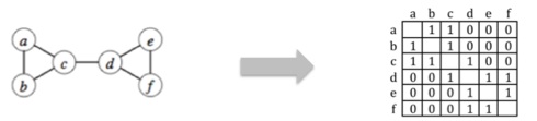
In graph theory, a network is described from nodes and connections. A network can also be represented as a square matrix with elements that represent the connections between each pair or regions. If there is no directionality defined for the connections, the matrix is symmetric. In brain imaging, nodes represent brain regions specialised to a specific task. Connections are represented as scalar values that measure 'strength’ either in structural data or in functional data. Defining the appropriate measure to describe 'strength’ is under investigation. In structural data, it reflects the capacity of the connections to transit a signal and it is therefore associated with fiber density, fiber packing and fiber integrity. In functional data, connectivity is associated with the degree of synchronicity of the signal between two regions and it is usually estimated based on correlation approaches.
Regions of Interest
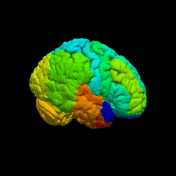
Atlas-based ROIs are defined very accurately based on anatomical landmarks, which are manually segmented to provide a set of regions, as shown at the figure on the right hand side. Although manual segmentation is prohibitively time-consuming, there are automated ways to propagate the segmentation from one subject to another. This involves non-rigid registration of the manually segmented images to the new. Altas-based segmentation is merged with tissue segmentation to provide ROIs in gray matter. Note, that atlas-based ROIs do not reflect accurately functional specialisation of the regions.
Connectivity-based ROIs can be derived based on either structural connectivity data from DWI or functional connectivity data from fMRI. The main concept is that the neurons that fire together they have similar functionality and thus they are also wired in a similar manner. Therefore, connectivity-based ROIs can be identified based on clustering approaches that group together voxels with similar connectivity profile.
Whole brain connectivity description
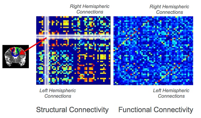
A connectivity matrix is a compact and systematic way to represent a brain network. For example, whole-brain structural connectivity matrices show direct structural connections between each pair of cortical regions. We choose to plot ROIs by cerebral hemispheres, with right-hemispheric ROIs in the lower left quadrant, left-hemispheric ROIs in the top right quadrant, and inter-hemispheric connections in the upper left and lower right quadrants. The colormap reflects the strength of each connection with deep blue representing the smaller values and red the highest values. Deep blue represents zero for structural connectivity or negative values for anti-correlated functional connectivity. The off-diagonal elements that appear as parallel lines to the main diagonal are inter-hemispheric connections between homologous regions.
Indirect Functional Connectivity
Although, we have characterise functional and structural connectivity with a similar form, a symmetric square matrix, yet there is still a fundamental difference: The absence of a structural connection does not correspond to the absence of a functional connection. We can observe synchronised activity between two regions even when there is no direct structural link that connects them. In this case, they are connected indirectly via one or more other regions. We call this indirect functional connectivity.
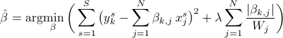
We can use the partial correlation matrix to disentangle the influence of other regions on a connection. Partial correlation matrix can be estimated from correlation matrices with inversion to derive the precision matrix and subsequently scaling the diagonal to one. In this context, the absence of a functional connection corresponds to the absence of a structural connection and vice-versa. Note that inversion requires a well-conditioned matrix with non-zero eigenvalues. Recall that inversion of zero is infinity and similar singularities can be observed when we invert a matrix.
A Gaussian Graphical Model
As the number of regions grows, it becomes more difficult to estimate a precise, well-conditioned covariance matrix. Well-conditioned refers to the intrinsic property of the correlation matrices to have positive eigen values. This is of paramount importance for the inversion of the correlation matrix to derive the partial correlation matrix.
To obtain a better-conditioned covariance matrix the time-series are modelled based on Multivariate Autoregressive Models (MAR). MAR models interregional dependencies within the data, taking in consideration the time influence one variable has on another. This is different from regression techniques that quantify instantaneous correlations. Here, we consider the functional brain activity as a stationary process and we use a zero-lag MAR model:
 , ,  is the number of regions and is the number of regions and  the time points corresponding to the fMRI volumes. the time points corresponding to the fMRI volumes.
 is a matrix specifying the connections between variables that can be understood as transition probabilities that reflect conditional independence. is a matrix specifying the connections between variables that can be understood as transition probabilities that reflect conditional independence.  is the identity matrix and is the identity matrix and  is Gaussian noise.
Stationarity implies that the distribution of the signal does not change with time and therefore has similar mean and variance over time. is Gaussian noise.
Stationarity implies that the distribution of the signal does not change with time and therefore has similar mean and variance over time.
Gaussian graphical models provide a graph representation of relations between random variables. Here we represent the interrelationship between fMRI time-series as a undirected graph with nodes/components representing the average fMRI signal within a set of regions. The graph edges describe conditional independence relations between the nodes. The conditional independence relations between components correspond to zero entries in the inverse covariance matrix, precision matrix.
Specifying the graph topology of a Gaussian graphical model is therefore equivalent to specifying the sparsity pattern of the inverse covariance matrix.
Estimation methods for Gaussian graphical models extend to solving autoregressive Gaussian processes.
To restrict the topology of the Gaussian graphical model and reduce the number of parameters, we inject prior knowledge based on the structural data. Recall that in the partial correlation context the absence of a structural connection corresponds to absence of the corresponding functional connection. We can select which connections to remove based on a t-test on each structural connection across the overall population of subjects.
Functional Connectivity as a Multivariate Object
Correlation matrices have specific mathematical properties:
Their diagonal elements are always ones (correlation of a time series with itself is always one).
They are symmetric (the correlation of a time series  with another with another  is the same as the correlation between and ). is the same as the correlation between and ).
They are positive definite, which implies they have positive eigenvalues.
The geometrical interpretation of a symmetric positive definite (SPD) matrix is simple when we consider two dimensional covariance matrices. Let say that a set of 2D points is given. Second order statistics describe their location with an ellipse (ie. PCA). The long axis of the ellipse is in the direction of the highest variance. The short axis is in the dimension of the lowest variance. The eigenvalues of the system correspond to the long and short axis of the ellipse. Therefore, it is not meaningful to have negative values.
Note that the prediction of each functional connection independently results in an unconstrained matrix that does not represent correlation. This results in a system, which is underpowered to detect interactions between function and structure over several regions.
We suggest to decompose the precision matrix:
This cholesky decomposition results in a matrix  that we can use for prediction, so that the reconstructed matrix that we can use for prediction, so that the reconstructed matrix  is always SPD.
It turns out that is the interaction matrix, which is also related to the connectivity matrix, is always SPD.
It turns out that is the interaction matrix, which is also related to the connectivity matrix,  . .
Therefore, cholesky decomposition is not just an abstract mathematical manipulation but it has an intuitive interpretation in the context of modelling the time-series with autoregressive models.
Stability Selection
LASSO is limited in that:
We extend this approach to randomized Lasso. The benefit is that the results are not sensitive to the parameters of the regression equations. Note that we have one parameter for each functional connection,  .
Randomised LASSO is a straightforward extension of LASSO and it is implemented, simply, by perturbing .
Randomised LASSO is a straightforward extension of LASSO and it is implemented, simply, by perturbing  randomly thousands of times.
The randomness is controlled by randomly thousands of times.
The randomness is controlled by  : :
Note that each of the extracted structural connection is associated with a probability. This probability is equal to the number of times the underlying connection was selected divided by the total number of LASSO repetitions.
Multiple Regression Analysis
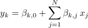
We suggest a prediction framework to study the link between structural brain connectivity and functional brain connectivity. A key advantage of this approach is that it describes influences of brain structure on function within a rigorous statistical framework. This data driven approach does not depend on a-priori hypothesis and thus, can facilitate the development of robust connectivity-based biomarkers. In this framework, each functional connection, is a dependent variable, which is described as a linear combination of  structural connections structural connections 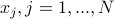 , also called independent variables or prediction variables. The goal is to estimate the , also called independent variables or prediction variables. The goal is to estimate the  parameters that provide the best least square fit over all subjects, parameters that provide the best least square fit over all subjects,  , of the linear equation: , of the linear equation:
Multiple regression is a statistical method for studying the relationship between a single dependent variable and several independent variables. It is used both for prediction and causal analysis:
In a prediction the goal is to construct a mathematical formula that estimates the dependent variable based on the observed independent variables.
In a causal analysis the independent variables are considered as causes of the dependent variable. The aim of the study is to detect whether a particular independent variable affects the dependent variable and to estimate the magnitude of this effect, if any.
Multiple regression is extremely popular in several sciences including social sciences, psychology, biology and clinical science. This is because:
In prediction studies, multiple regression makes it possible to combine many variables to produce optimal predictions of the dependent variable.
In causal analysis, it separates the effects of independent variables on the dependent variable so that you can examine the unique contribution of each variable.
Although, multiple regression is based on a linear equation, it can describe complex relationships between structure and function. In the absence of any prior knowledge, a linear equation is the simplest way to describe a relationship between structure and function and still get reasonably accurate predictions. Note that in multiple regression the dependent variables can also take non-linear forms. Here, we are not going to explore this further.
Also note that multiple regression analysis can analyse any dataset tailored for ANOVA, whereas the opposite is not always true. It yields identical statistical tests to those provided by ANOVA yet it offers additional measures of effect size and it often permits more straightforward interpretation.
Sparse Multiple Regression Analysis
Evidence that the relationship between functional and structural connectivity is sparse come from recent work in traumatic brain injury that shows that the integrity of a structural connection, between the right anterior insula and the pre-supplamentary motor area, predicts function within the default mode network, exclusively (Bonnelle et al., PNAS, 2012).
A sparse representation over least square multiple regression it offers two major advantages that are very useful in modelling brain connectivity:
It improves prediction by setting some coefficients to zero. This results in removing noisy and irrelevant variables and thus reducing the total variance.
It allows the selection of the most relevant variables and thus it links each functional connection with a subset of structural connection in a data driven way.
We use the Least Absolute Shrinkage and Selective Operator (LASSO) to impose an  penalty on the multiple regression that controls its sparsity. LASSO can be implemented with computationally efficient ways and it controls sparsity with just one parameter, . When gets high values most of the coefficients are set to zero and the corresponding structural connections are eliminated. The remaining structural connections are those strongly linked with the functional connection : penalty on the multiple regression that controls its sparsity. LASSO can be implemented with computationally efficient ways and it controls sparsity with just one parameter, . When gets high values most of the coefficients are set to zero and the corresponding structural connections are eliminated. The remaining structural connections are those strongly linked with the functional connection :
The correct predictors are identified with high probability even when the number of variables is higher than the number of observation under the assumption that functional brain connectivity can have a true sparse representation based on structural connectivity.
Source Code
MapFunctionOnStructure GitHub Repository
Acknowledgements
The last two years I have been collaborating with the Parietal team, INRIA, FRANCE. The key suggestions on how to regularise the correlation matrices, the implementation of the Gaussian graphical model and the transition from LASSO to randomised LASSO comes from Dr. Gael Varoquaux.
The Computational, Cognitive and Clinical Neuroimaging Laboratory (C3NL) and in particular Dr David Sharp and Dr Robert Leech provided us with data and advice on connectivity-based ROIs.
Christian Ledig for helping with atlas-based segmentation.
Dr. Emma Robinson for providing the software to estimate the strength of structural connections.
Prof. Christian Beckmann for advice on sparse multiple regression and indirect connectivity.
Prof. David Edwards for recognizing early the importance of combining structural connectivity and resting-state functional connectivity.
Prof. Daniel Rueckert for the overall supervision and advice on a prediction framework and non-rigid registration. The project has been benefited from several registration tools.
This project was funded from an MRC fellowship award (G0701782).
Related Publications
F. Deligianni, G. Varoquaux, B. Thirion, D.J. Sharp, C. Ledig, R. Leech and D. Rueckert, A Framework for Inter-Subject Prediction of Functional Connectivity from Structural Networks, IEEE Trans on Med Imaging, in press.
F. Deligianni, G. Varoquaux, B. Thirion, E. Robinson, D.J. Sharp, A. D. Edwards and D. Rueckert, Relating brain functional connectivity to anatomical connections: Model Selection, NIPS-MLNI, 2011. pdf
F. Deligianni, G. Varoquaux, B. Thirion, E.Robinson, D.Sharp, A.Edwards, and D.Rueckert, A Probabilistic Framework to Infer Brain Functional Connectivity from Anatomical Connections, IPMI, 296-307, 2011. pdf
F. Deligianni, E. C. Robinson, C. F. Beckmann, D. Sharp, A. D. Edwards, and D. Rueckert, Inference of Functional Connectivity from Direct and Indirect Structural Brain Connections, ISBI, 849-852, 2011. pdf
F. Deligianni, E. C. Robinson, C. F. Beckmann, D. Sharp, A. D. Edwards, and D. Rueckert, Inference of Functional Connectivity from Structural Brain Connectivity, ISBI, 1113-1116, 2010. pdf
|